Saving lives with data: Oslo's journey in ambulance demand forecasting
Time series forecasting has several applications and can provide valuable information. Recently I worked on a project forecasting ambulance demand for the emergency medical dispatch in Oslo. Using machine learning, statistical methods and a combination of the two, we explored how to forecast the demand as accurately as possible. The aim of this article is to give a general introduction to the process we used to create these models, which I believe can be relevant for many other applications as well.
5 min read
·
By Erling Van De Weijer
·
December 24, 2023

Forecasting ambulance demand is critical for emergency medical services to allocate their resources as efficiently as possible. One year ago, working with Oslo University Hospital and their emergency medical dispatch, I worked on a project to create a forecasting model for the ambulance demand in and around Oslo. Our goal was to give the ambulance dispatchers a clearer understanding of when and where there likely will be demand for ambulances, to aid their decision making in placing and dispatching ambulances.
Based on previous research, we created one model for predicting the number of dispatches at a given time slot which we will refer to as the volume. We create a separate model for predicting the spatial distribution or in other words the geographic location of the incidents demanding an ambulance are. The overall idea, is that it is better to have two models solve two separate and simpler problems, in this case volume and distribution, rather than one model on one difficult problem which would be the combination of the two. This article focuses on the volume forecasting model.
In order to forecast the volume, we group the gathered data into a time series. A time series is sequence of data points indexed with a time of equal interval lengths. For this problem, we use hourly intervals, and the corresponding data point refers to the number of ambulance dispatches for that given hour. Time series forecasting, is the art of predicting the value, in this case the number of ambulance dispatches required, for future time periods.
Our data set consisted of several data points for all events received by the medical dispatch unit over a three year period. These events were grouped into hourly intervals, resulting in a time series ready for predictions!
Initial data analysis
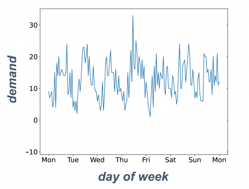
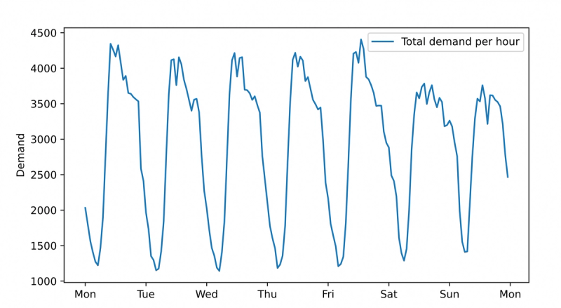
The images below shows som early data visualisation we generated to get a better understanding of the time series we worked on.


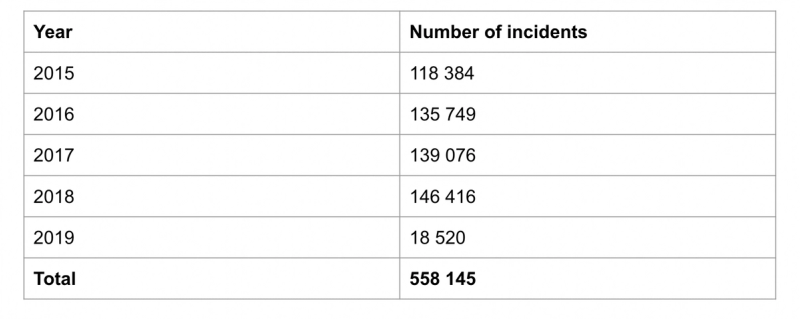
Examining the time series above, we can see that during the day there are more events than during the evening. Additionally, there seems to be slightly more incidents during friday and saturday evening while having lower peaks during the day, compared to the other days of the week. From this, we can deduct that the ambulance demand follows some patterns based on the time of day, as well as day of the week. Interesting! What else can we learn just by visually examining our data? Well, let us put the annual demand into a table, to see if we can see another pattern.

Inspecting the table, we can see that every year the ambulance demand increases.
Creating a forecasting model
Ahead of our project, there was already done some published research on using neural networks and machine learning to forecast the same problem, using the same data set. Our goal, was to create models that could provide more accurate forecasts than previous models. Like previous work, we wanted to use neural networks, since they have proven to be a state of the art tool for time series forecasting. So, what can we do to improve provide more accurate forecasts than previous machine learning models?
Based on initial data analysis, we knew that the time series followed two patterns. One is the weekly pattern, where the average volume is based on the day of the week, as well as the time of day. The other is the yearly steady increase in demand. What if we could extract this information from our time series, resulting in a less complex time series for our machine learning model to forecast.
Well, this is what inspired our model architecture. Using tools from statistical decomposition, we could simplify the time series. We experimented using both singular spectrum analysis and seasonal trend decomposition using LOESS, for this purpose. Using these tools we could extract the two patterns mentioned above, namely the seasonality and trend in the time series. Using regression, we could also predict what these values would be in future events. We trained a neural network on what was left after decomposition, and used the trained network to predict future values. The final predictions, consisted of the sum of the predicted values of these models.
Results and reflections
Our final models, combining statistical decomposition and neural networks, outperformed previous models using only neural networks. This confirmed our suspicion, that simplifying the time series before applying machine learning, resulted in more precise predictions.
So, how can these resulted be translated to other applications? Looking at the bigger picture, this illustrates the benefits of analysing a problem before trying to solve it. By breaking it down to smaller, simpler problems and using the right tools to solve each of these problems, we could make more precise forecasts. This also applies when using machine learning, even though one would believe they could learn this problem area without simplifying the time series.
If you are interested in learning more details about the details of these models or the project, I co-wrote a published research article, that is linked to below, that goes into the technical details of our models.
Up next...
Loading…